The natural world is full of complex group behaviours. Birds flock, fish school, and ants march in lines. Even plants, some microbes, and plankton exhibit group behaviours. These behaviours can usually be modeled, and are often relevant to the ecological interactions and spatial distribution of the species that exhibit them. In this short series, we’ll implement Boids, a common agent-based model of schooling behaviour in fish and birds in QGIS, a popular open source GIS platform. This is part 1 of the series, the introduction and contents post. Click here for part 2.
You can also check out the code for this on my github.
Contents
- Introduction (you are here)
- A note on testing
- Layout and constraints
- Primary behaviours
- Putting it all together
- Enforcing speed limits and study area constraints
- Implementation in QGIS
What is an ABM?
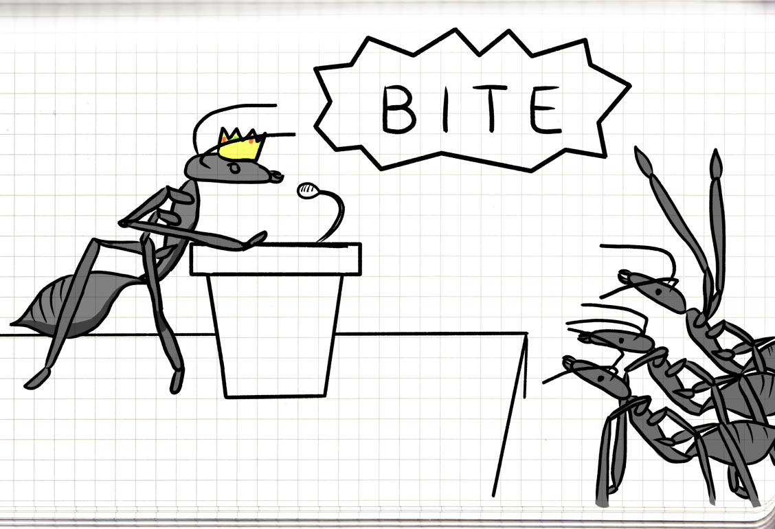
Some birds, fish, and virtually all ants all exhibit a high degree of group spatial organization in their day to day activities. How do birds know to flock, fish know to school, and ants know to march in lines to the still-living grasshopper they are gruesomely dismembering? In the case of ants, the answer is obvious. Ants, like all eusocial hymenopterans observe an absolute monarchy. They simply do whatever the queen asks!

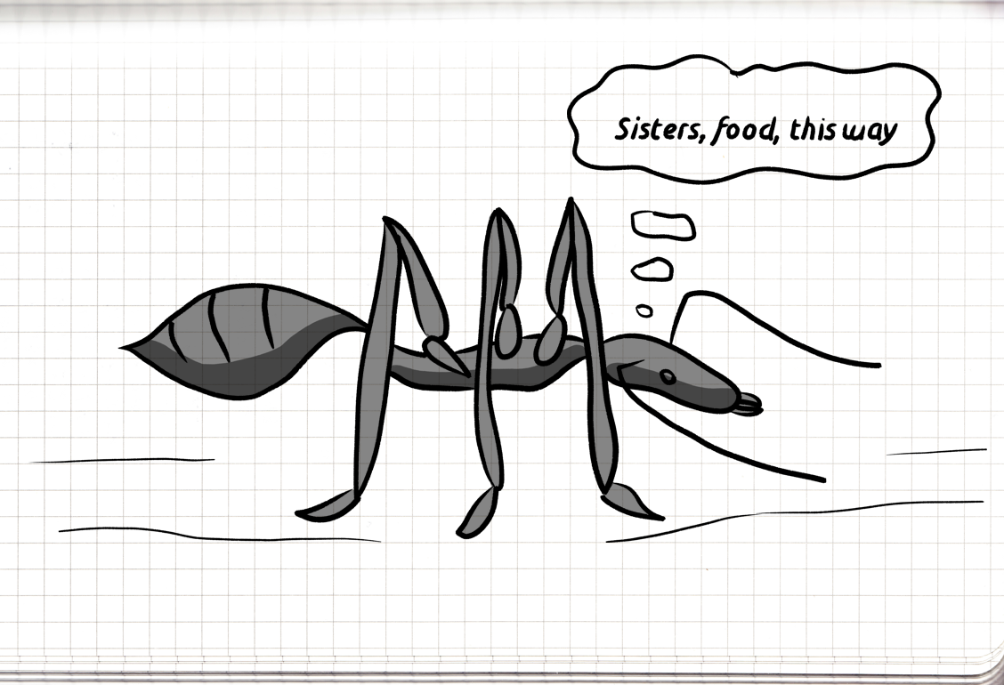
Of course, we know this is far from the truth. Most ant species communicate primarily through scent, and where George Lucas’s Jawas seem to be able to communicate complex ideas this way, it doesn’t seem like most Earth creatures can communicate that well using scents. The queen of many species can adjust the general behaviours of the colony through pheremones, but the ants seem to mostly organize by labeling their environment by leaving scent trails for other ants to follow.

A convincing model of ant behaviour can be constructed as follows:
If not carrying food:
    examine environment
    if food at location, pick up food
    else if food nearby, orient on food
    else if trail to food nearby, orient on trail
    else choose a direction randomly
    move in chosen direction
    leave trail to colony
If carrying food:
    examine environment
    if colony at location, drop food
    else if colony nearby, orient on colony
    else if trail to colony nearby, orient on trail
    else choose a direction randomly
    move in chosen direction
    leave trail to food
We can instantiate some large number of these models in an environment that contains a colony and a food and simply loop through running the code of each ant:
Colony = [x, y]
Food = [x, y]
Ants = [ant(colony) for _ in range(1000)]
while 1:
    for ant in ants:
        Do ant behaviours
This is a spatially explicit agent based model (ABM). Seriously, that’s all there is to it. The ant object is an agent, while the script that instantiates a bunch of ants and calls their behaviours is a control or environment script. In similar ant models (you usually need to make the trails fade over time to avoid overrunning the area with trails), the ants will swarm until some find the food source, then establish the characteristic trails to the food source that we have all observed in nature. Over time the trails become straighter as the scents of the initial meandering paths that the ants took to get to the food are overwhelmed by stronger, better oriented scent trails. Marching in lines is an emergent behaviour arising from the simple orientation rules and sensory systems of the individual ants.
Guidelines for building ABMs
We aren’t stuck with ants, ABMs can be used to model any number of different structures. We’re going to abandon the ants example here and move on to schooling behaviour, but you can model any group action, from economic decision making to the spread of contagious illnesses using ABMs. Agents and control scripts can be as complex or as simple as we feel is justified, but we will always have those two components: an agent model, responsible for implementing the behaviours of the animal, plant, or object we are studying; and a control or environment model that instantiates the agents, tracks time, and tracks any relevant environmental data. Agent-based models are almost always run in discrete time, and can be spatially explicit. Spatially explicit agent-based models can be run in discrete or continuous space. We are going to work in continuous space here, but many habitat models are run in discrete space (The USDA Forest Service’s inStream trout model, for example, simulates trout as being in discrete locations within a grid of habitat areas in a river). Choosing the correct model for our system is the first step in getting reproducible results that can be validated.
Some other general guidelines for building ABMs:
- Models should be parsimonious—As with all models, when we have two competing models that make the same predictions, the simplest model is usually correct.
- Models should make testable predictions—If we want to use our model as a representation of an actual system, we need to be able to verify that our results imitate nature to the point of being useful.
- Models should be agent-driven—Wherever possible, complex group patterns should be emergent properties arising from simple individual behaviours from our agents. Animals are typically limited by their sensory abilities, and often don’t employ complex communication strategies.
Can we think of an agent that implements schooling behaviour in fish? A naive approach might look like:
if in school, follow school
if not in school, steer toward school
How does our fish know if it is in a school though, especially if it has limited vision and can’t receive planning information from a leader? Fish schools don’t have teachers, after all. In this short series we are going to focus on the boids model, developed by Craig Reynolds in 1986. Reynolds is an artificial life expert who was focused on simulating flocking behaviours in birds for computer animation. His agent-based model has formed the basis for simulations of schooling behaviours in fish, flocking behaviours in birds, and herding behaviours in ungulates.
What is a boid?
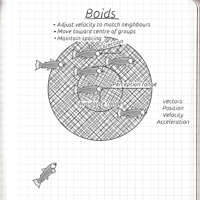
In 1986, artist and artificial life expert Craig Reynolds, whose work you might know from Tron (1982); Batman Returns (1992); or Flocks, Herds, and Schools: A Distributed Behavioral Model (Reynolds 1987), created bird-oid objects. Boids were originally intended to simulate flocking behaviours in birds and the model as a whole is composed of an arbitrary number of agents who exhibit three simple behaviours. Each boid agent has a position, velocity, and acceleration. The model operates in continuous space and in discrete time, and each time step the boid updates its position by adding its velocity to its position, updates its velocity by adding its acceleration to its velocity, and computes a new acceleration based on what is necessary to meet its behavioural objectives.

The three behaviours that the boid uses to compute its acceleration are alignment, cohesion, and separation (or avoidance). Alignment is a behaviour where the boid will attempt to adjust its velocity to match the velocity vectors of nearby boids. Cohesion is a tendency for the boid to attempt to move toward the centre of any nearby boids. Separation is a behaviour where the boid will attempt to avoid colliding with or crowding nearby boids. Flocking, or schooling in fish (I’m going to call it schooling from here on because I am a fish biologist) is an emergent behaviour that results from the three primary behaviours. In pseudocode:
locate boids within sensory range
alignment: steer in the same direction as nearby boids
cohesion: steer toward the center of the group
separation: steer away from any boids that are too close
accelerate in the resultant direction
Boids can accomplish schooling behaviours with limited sensory ranges (they don’t need to be able to see much past their own avoidance range and don’t need to be able to perceive the entire school), and with only the ability to determine the position and velocity of other boids.
Our setup
We’re going to implement our boids in Python (3.x) for use in a QGIS (3.x) plugin. I’m not a huge fan of Python, but close integration with the best extant GIS software is perhaps worth dealing with slow processing and a frankly hideous lack of brackets and semicolons. We will use NumPy to handle our vectors, but won’t depend on anything else for the model itself. We’re also going to implement our vectors in 2 dimensions because this is an educational exercise that doesn’t represent reality. If you decide to use this model for actual science, you will need to add a dimension, which is easy; and figure out where the bottom is, which is hard.
